
The long Period
The long period is defined as the period that is long enough for the inputs of all factors of production to be varied. In this period no factor is fixed, all are variable factors. Firm has enough time to change its scale of production. It can purchase and install new machinery or it can sell the old one; it can vary the size of factory; it can increase or decrease the number of even permanent employees of the firm. Thus in long run all sorts of changes in the factors of production are possible.
AS all costs are variable in the long run, the total of these costs of production. In the long run, only the average total cost is important and considered in taking long-term output decisions.
Long run average costs are per unit cost of production at different levels of output by change the size of plant or scale of production. The main point here is that any cost remains long run cost till a new level of output is achieved and as soon as a new level of output is achieved, the long run costs become short run costs.
The long-run cost-output relationship is depicted graphically by the long-run cost curve-a curve depicting how costs will change when the scale of production is varied.
The concept of long-run costs can be further elaborated with the help of an illustration. Assume that at a particular time a firm operates under average total cost curve U2 and produce OM output. Again, it is desired to produce ON amount. If the concern continues under the old scale, its average cost will be NT. If the scale to the firm is changed, the new cost curve will be U3 The average cost of producing ON will then be NA. NA is less than NT. So the new scale will be preferable to the old one and should be adopted.
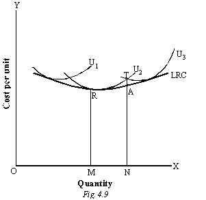
In the long run, the average cost of producing ON output is NT. This we can say as the long run cost producing ON output. We must be careful here to note that we shall call NA as the long run cost only so long as the U2 scale is in the planning stage and is not actually adopted. The moment the ale is adopted, the NA cost will be the actually short run cost producing ON output as shown is Fig. Below.
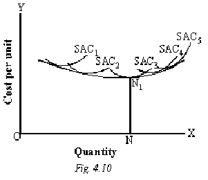
To draw the long run cost curve we have to commence with a number of short run average cost curves (SAC curves), each curve representing a particular scale of size of the plant including the optimum scale. One can now draw the long run cost that will be tangential to the entire family of SAC curves. It means that it will touch each SAC curve at one point.
Here, the assumption is that the number of possible short run curves is infinitely large i.e. a plant of virtually any size can be built. If however, we suppose that only, Limited say five, alternative size of plants are technically possible, the long run cost curve will be scalloped i.e., a wavy solid line consisting of lowest segments of all the short-run average cost curves.
