Equilibrium of a Firm
Equilibrium is a situation from where firm a firm does not want to deviate. Generally this happens when the firm is earning maximum profit since it is the most advantageous position, therefore the firm does not want to change its position. Thus it is the state of equilibrium. The equilibrium of a firm can be explained in two ways:
- Total Revenue and Total cost curves approach and
- Marginal Revenue and Marginal cost curves approach.\
- Total Revenue and Total Cost Curves Approach. Firm will be in equilibrium position at the level of output where its money profits is maximum. It can maximize its profits by producing at that particular level of output where the difference between total revenue and total cost is maximum. This can be explained with the help of a diagram.
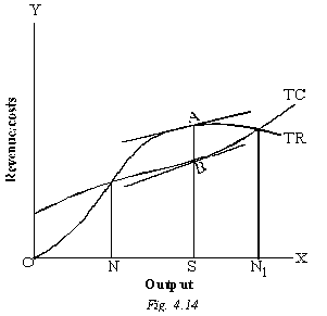
The above diagram shows that as long as the level of output is less than ON or greater than ON1′ total costs exceed total revenue and the firm is under loss. At both the levels of output i. e. ON and ON1 firm is neither having losses nor profits. Thus between N and N1 lie the point of equilibrium where firm can earn maximum profits to know the point draw two parallel tangents to TC and TR curves between N and N1 levels of output. In this way get the longest vertical distance at OS level of output. This gives us the point of maximum profits.
The main weakness of this method is that it is not possible to know the maximum vertical distance between TC and TR curves by more looking at the curves. Moreover this method does not tell us about the price of the product at the equilibrium point.
- Marginal Revenue and Marginal Cost Approach. A firm will come into equilibrium when two conditions are fulfilled. (i) The MR is equal to MC; and (ii) Mc must cut MR from below. We shall look into the equilibrium of firm when; (a) AR and MR are horizontal to X-axis and (b) AR and MR have downward slope form left to right.
- When AR and MR are horizontal. The figure given below the illustrate equilibrium of the firm.
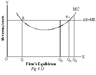
When AR is constant MR becomes equal to it. MR intersects MC at R and R1. At both these points MC is equal to MR. Point R can not be a determinate equilibrium point since beyond this point, the MC is lower than MR and it is advantageous to the firm to produce more. By doing of, the firm can secure profits shown by the area RKR1. The determinate equilibrium point is in fact OQ for beyond that point MC and MR is not a sufficient condition of a firms equilibrium and that it is necessary that the MC curve cuts the MR curve from below, so that beyond the position of equality of MC and MR. MC is more than MR.
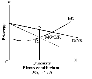
- AR and MR having downward slope. The following figure shows that the firm has a downward sloping demand curve or average revenue curve. The corresponding MR curve is also down sloping from left to right. The MC curve is rising. At point R marginal cost curve cuts marginal revenue curve from below. This is equilibrium position of the firm. The equilibrium quantity is OQ and the equilibrium price is OP. The firm cannot produce beyond OQ because the additional cost of production will be higher than the additional revenue. At the same time, the firm will not like to produce less than OQ because its profits will not be maximized except at OQ. Therefore, the firm is in equilibrium when MC = MR