The concept of multiplier – Macroeconomics

 

 

The concept of multiplier

The concept of multiplier was first developed by R.F. Kahn in his article “The Relation of Home Investment to unemployment” in the Economic Journal of June 1931. Kahn’s multiplier was the employment multiplier. Keynes took the idea from Kahn and formulated the Investment multiplier. So, the concept of multiplier is regarded as one of the important contributions of J.M. Keynes to economics. The economists before Keynes were not unaware of the effect of an increment in investment on the increment of income. For example, Knut Wicksell, for the first time, had used multiplier in the context of inflation. Similarly, N. Johanson had explained it in 1903. But, the economists before Keynes had not been able to explain the concept of multiplier in a clear way.

Keynes used the concept of multiplier in the form of investment multiplier. According to Keynes, “Investment multiplier tells us that when there is an increment of aggregate investment, income will increase by an amount which is K times of the increment of investment”, i.e., DY=K×DI, where Y is income, I is investment, D is change (increment or decrement) and K is the multiplier. Then the multiplier is expressed as;

K=  [ratio of change in income to the change in investment]

The multiplier expresses a relationship between an initial increase in investment and final increase in aggregate income. So, the multiplier theory shows that how many times the income increases as a result of an initial increase in investment or it is the ratio of an increase of income to given increase in investment. For example, if increase in investment is made by Rs. 10 lakhs. As a result, after some time period the total income increases to Rs. 50 lakhs. The income has increased by five times. Hence, the multiplier is 5. In the multiplier theory, the important element is the multiplier coefficient, K which refers to the power by which any initial investment expenditure is multiplied to obtain a final increase in income.

• Relationship Between the Multiplier and Marginal Propensity to Consume (MPC):

The value of multiplier is determined by the marginal propensity to consume. The multiplier is large or small according as the marginal propensity to consume is large or small. Thus, higher the marginal propensity to consume, the higher is the value of multiplier, and vice-versa. The relationship between the multiplier and the marginal propensity to consume is as follows:

 

Total Income (Y) = Total consumption (C) + Total Investment (I)

or,  Y = C+I

or,  DY= DC+DI

or,  DI =DY-DC —- ® (i)

Now,    by definition we know that

K=  or, DY= K. DI

or, DI =  —-® (ii)

Now substituting the value of DI from (ii) into (i), we get

= DY- DC —-®(iii)

Further, dividing (iii) by DY, we get

= 1 –  ——®(iv)

or, Inverting (iv), we get

K =  =  =

Since K stands for multiplier, DC/DY stands for marginal propensity to consume and 1- DC/DY stands for marginal propensity to save (MPS) The multiplier can also be derived from the marginal propensity to save (MPS) and it is the reciprocal of MPS, i.e., K=1/MPS. There is an inverse relation ship between multiplier and MPS. Higher the MPS, lower is the multiplier. Thus, the multiplier is directly related to MPC and inversely related to MPS.

From this formula, we can compute the various values of the multiplier corresponding to various ‘MPC’ as follows:

 

DC/DY (MPC) [1-MPS]	DC/DY (MPS) [1-MPC]	K (multiplier coefficient) [K= = ]
0	1	1
1/2	1/2	2
2/3	1/3	3
3/4	1/4	4
4/5	1/5	5
8/9	1/9	9
9/10	1/10	10
1	0	¥(infinity)

The table shows that the size of the multiplier varies directly with the MPC and inversely with the MPS. Since the MPC is always greater than zero and less than one (i.e., O<MPC<1), the multiplier is always between one and infinity (i.e., 1<K<¥). If the multiplier is one, it means that the whole increment of income is saved and nothing is spent because the MPC is zero. On the other hand, an infinite multiplier implies that MPC is equal to one and the entire increment of income is spent on consumption. It will soon lead to full employment in the economy and then create a limitless inflationary spiral. But these are rare phenomena. Therefore, the multiplier coefficient varies between one and infinity.

The process of multiplier operation can be shown in figure below:

 

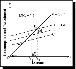
In the figure, the 45º line represents OY income curve. C is the consumption curve having a slope of 0.5 to show the MPC is equal to one-half. C+I is the initial consumption and investment curve, which intersects the 45º line at point E, so point E is initial equilibrium point where aggregate income is equal to aggregate demand (C+I), in this condition equilibrium level of income is OY₁.

Now, suppose that investment increases by DI, as a result C+I curve shifts upward to C+I+ DI curve. This curve intersects 45º line at the point E, which is the new equilibrium level where aggregate income also increased by DY level of income, i.e., which is double than the increase in investment.

Multiplier works both in the forward direction as well as in the backward direction. If investment decreases, the multiplier operates in the reverse direction. A reduction in investment leads to contraction in income and consumption which causes cumulative decline in income. On the other hand, if consumption and investment increases, the multiplier operates in the positive direction. Thus, higher the MPC, the greater is the value of the multiplier and vice-versa.