Monopoly – Imperfect Competition – Monopolistic Competition

Features of Monopoly

  1. There is only one firm or producer of product having no close substitutes.
  2. A monopolist can fix the price of his product as he likes. He is therefore a price maker.
  3. The goal of monopolist is to seek maximum total profit not ‘maximum unit profit”.
  4. The firm is industry in case of monopoly. There is no need to separate the firm from the analysis of industry.
  5. Entry of other firms is restricted in monopoly.

Forms of Imperfect competition

Since imperfect competition refers to the entire situation between perfect competition and monopoly, there connote be only one certain form of it. Normally following market conditions are referred to when we talk to imperfect competition.

  1. Monopolistic Competition.
  2. Oligopoly
  3. Absence of pure monopoly.

Because the brief discussion of these varied forms of imperfect competition it would be proper to know the dissimilarities between imperfect competition and monopolistic competition.

  1. Imperfect competition is a negative concept; what is not perfect is imperfect. As such it has a wide connotation. Monopolistic competition on the other hand is a positive concept. It shows the existence of competition but qualified by monopolistic elements.
  2. Chamber shows the importance of product differentiation and of selling cost under monopolistic competition. Each firm is producing a different variety of a product and each is resorting to advertisement in order to push up its sales. Under imperfect competition these aspects are ignored.

Features and Causes of Monopolistic Completion

  • Under monopolistic competition, the product will not be identical or homogeneous and at the same time will not be entirely different form each other. The products are differentiated and are commonly known by brand names or trademarks. There will be competition between rival brands of each product. The consumers may come to acquire special preferences for particular brands.
  • Monopolistic Competition is characterized by imperfections in the market which may arise due to ignorance, inertia, cost of transport, irrational ignorant about the availability and the prices of the different brands in the market. Similarly sellers too may not have equal knowledge about the market and the prices in the different sections of the market.
  • A large number of sellers. In a monopolistic competitive market, the number of sellers is large (but not as many as imperfect competition) and they are not dependent on rivals, actions. They act quite independently without caring for their rivals.
  • Competition. As because each prouder or seller is independent in his actions, but each one takes decisions, considering others’ actions and their effects on buyer’s behavior. This situation leads to competition among sellers. The producers or sellers never work in collusion with each other.
  • Free Entry and Exit. Like perfect competitive situation, there is perfect freedom for firms to enter or leave the industry at any time. They have to face a number of problems in entering the market under monopolistic conditions as competed to, perfect competition.

TYPES OF MICRO ECONOMICS

  1. TYPES OF MICRO ECONOMICS

The analysis of microeconomics is always affected by time period. But there are still some economists who do not believe the time value in microeconomics analysis. Based upon the equilibrium of microeconomics in the different situation and relationship between time and different economic models, the microeconomics is divided into three different types, namely Microsatics, Comparative Micro statics and Micro Dynamics.


  1. Micro Statics:

Demand and supply are two principal variables that determine the equilibrium level for market. The quantity demanded of a good at a time is generally considered to be related to the price of that particular time. Same way supply is also related to price at particular static time. Thus microeconomics tries to find out the equality of demand and supply at a particular point of time or static time. This static analysis is the study of static relationship between two variable called demand and supply, which is known by micro statics. In other words, if the functional relationship is established between two principles variable at a same period of time, such analysis is known by micro static. This situation is also known by equilibrium situation of variables. This equilibrium determines the equilibrium price and quantity. According to Schumpter, “By static analysis, we mean, method of dealing with economic phenomena that tries to established relations between elements of the economic systems-prices and quantities of commodities all of which have the same time subscript, that is to say, refer to the same point of time.” He further said, “Static analysis tries to establish relation between elements of the economic system which refer to the same point of time.”


The concept of micro static is given below with the help of diagram.

In the diagram given above, DD shows demand curve and SS shows supply curve. Both curves intersect at point ‘E’ that gives the equilibrium price- P and quantity- Q at particular time period. This is static analysis.


  1. Comparative microstatics:

Micro static explains about the equilibrium point that is obtained by two co- operant factors that is demand and supply, under the static or given period of time. Thus equilibrium is obtained when demand equals supply under the condition of ‘other things remaining same’ or ‘no change’. When variables change, the initial equilibrium level will be disturbed. This brings the process of disequilibria and it continues till new equilibrium is obtained. In this background it is essential to analyze the comparison between these two equilibrium levels. The comparison between these two different equilibriums is studied under comparative microstatics. It compares one equilibrium with other equilibrium but does not identify the process of disequilibria that occurs. According to Prof. Schneder; “The comparative analysis of two equilibrium positions may be defined as comparative static analysis. Since, it studies the alternation in the equilibrium position corresponding to an alternation in a single datum.”


For example, suppose that income of consumer changes that affects to demand of consumer and regarding supply, initial equilibrium distributes and new equilibrium is obtained. Same way due to change in the technology, production function, then cost and hence supply change and this affects the initial equilibrium. Thus in both cases- either demand changes or supply changes, two equilibrium appear- initial and later. Comparative micro statics studies those two equilibriums.


The diagram given explains the comparative micro statics equilibrium. In the diagram, demand curve DD and supply curve SS gives the equilibrium point ‘E’ at price- P and quantity- Q. due to changes in the demand, it shifts to D1D1 and new equilibrium point ‘E1’ is obtained with the same supply curve SS. This new equilibrium gives new price- P1 and quantity- Q1. Comparative micro statics studies the two equilibrium points ‘E’ & ‘E1’.


  1. Micro dynamics

Study of microstatics shows the state of equilibrium through demand supply analysis under the assumption of constant time where no changes in variables take place. Same way study of comparative micro statics shows the comparison between two equilibriums due to partial change in factors and time period. But the world and time are neither static nor they partially change. The real world is dynamic. The change in time and other factors are dynamic and they lead to change in demand and supply hence change in equilibrium. Thus micro dynamics refer to a position by which the system passes from one position of equilibrium to other. It is very essential to know change and process of change in equilibrium. In this analysis with the change in pace of time price of commodity also changes and that brings the change in demand and supply. Those changes bring the true picture of real world economy at different prices at different time. According to J.A. Schumpeter, “we call a relation dynamic if it connects economies quantities that differ to different points of time.” W.T. Bauomol said, “Economic dynamics to the study of economic phenomena in relation to preceding and succeeding events.” The other most important aspect of micro dynamic is that it deals with disequilibria condition also. The analysis chases process of change time by time. It can explain state of being disequilibria and how the disequilibria’s move towards equilibrium.

The concept of multiplier – Macroeconomics


The concept of multiplier

The concept of multiplier was first developed by R.F. Kahn in his article “The Relation of Home Investment to unemployment” in the Economic Journal of June 1931. Kahn’s multiplier was the employment multiplier. Keynes took the idea from Kahn and formulated the Investment multiplier. So, the concept of multiplier is regarded as one of the important contributions of J.M. Keynes to economics. The economists before Keynes were not unaware of the effect of an increment in investment on the increment of income. For example, Knut Wicksell, for the first time, had used multiplier in the context of inflation. Similarly, N. Johanson had explained it in 1903. But, the economists before Keynes had not been able to explain the concept of multiplier in a clear way.

Keynes used the concept of multiplier in the form of investment multiplier. According to Keynes, “Investment multiplier tells us that when there is an increment of aggregate investment, income will increase by an amount which is K times of the increment of investment”, i.e., DY=K×DI, where Y is income, I is investment, D is change (increment or decrement) and K is the multiplier. Then the multiplier is expressed as;

K=  [ratio of change in income to the change in investment]

The multiplier expresses a relationship between an initial increase in investment and final increase in aggregate income. So, the multiplier theory shows that how many times the income increases as a result of an initial increase in investment or it is the ratio of an increase of income to given increase in investment. For example, if increase in investment is made by Rs. 10 lakhs. As a result, after some time period the total income increases to Rs. 50 lakhs. The income has increased by five times. Hence, the multiplier is 5. In the multiplier theory, the important element is the multiplier coefficient, K which refers to the power by which any initial investment expenditure is multiplied to obtain a final increase in income.

  • Relationship Between the Multiplier and Marginal Propensity to Consume (MPC):

The value of multiplier is determined by the marginal propensity to consume. The multiplier is large or small according as the marginal propensity to consume is large or small. Thus, higher the marginal propensity to consume, the higher is the value of multiplier, and vice-versa. The relationship between the multiplier and the marginal propensity to consume is as follows:


Total Income (Y) = Total consumption (C) + Total Investment (I)

or,  Y = C+I

or,  DY= DC+DI

or,  DI =DY-DC —- ® (i)

Now,    by definition we know that

K=  or, DY= K. DI

or, DI =  —-® (ii)

Now substituting the value of DI from (ii) into (i), we get

= DY- DC —-®(iii)

Further, dividing (iii) by DY, we get

= 1 –  ——®(iv)

or, Inverting (iv), we get

K =  =  =

Since K stands for multiplier, DC/DY stands for marginal propensity to consume and 1- DC/DY stands for marginal propensity to save (MPS) The multiplier can also be derived from the marginal propensity to save (MPS) and it is the reciprocal of MPS, i.e., K=1/MPS. There is an inverse relation ship between multiplier and MPS. Higher the MPS, lower is the multiplier. Thus, the multiplier is directly related to MPC and inversely related to MPS.

From this formula, we can compute the various values of the multiplier corresponding to various ‘MPC’ as follows:


DC/DY (MPC)

[1-MPS]

DC/DY (MPS)

[1-MPC]

K (multiplier coefficient) [K= = ]
0 1 1
1/2 1/2 2
2/3 1/3 3
3/4 1/4 4
4/5 1/5 5
8/9 1/9 9
9/10 1/10 10
1 0 ¥(infinity)

The table shows that the size of the multiplier varies directly with the MPC and inversely with the MPS. Since the MPC is always greater than zero and less than one (i.e., O<MPC<1), the multiplier is always between one and infinity (i.e., 1<K<¥). If the multiplier is one, it means that the whole increment of income is saved and nothing is spent because the MPC is zero. On the other hand, an infinite multiplier implies that MPC is equal to one and the entire increment of income is spent on consumption. It will soon lead to full employment in the economy and then create a limitless inflationary spiral. But these are rare phenomena. Therefore, the multiplier coefficient varies between one and infinity.

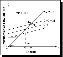
The process of multiplier operation can be shown in figure below:

multiplier


In the figure, the 45º line represents OY income curve. C is the consumption curve having a slope of 0.5 to show the MPC is equal to one-half. C+I is the initial consumption and investment curve, which intersects the 45º line at point E, so point E is initial equilibrium point where aggregate income is equal to aggregate demand (C+I), in this condition equilibrium level of income is OY1.

Now, suppose that investment increases by DI, as a result C+I curve shifts upward to C+I+ DI curve. This curve intersects 45º line at the point E, which is the new equilibrium level where aggregate income also increased by DY level of income, i.e., which is double than the increase in investment.

Multiplier works both in the forward direction as well as in the backward direction. If investment decreases, the multiplier operates in the reverse direction. A reduction in investment leads to contraction in income and consumption which causes cumulative decline in income. On the other hand, if consumption and investment increases, the multiplier operates in the positive direction. Thus, higher the MPC, the greater is the value of the multiplier and vice-versa.

Measures to Raise the Propensity to Consume


Measures to Raise the Propensity to Consume

In the short period due to psychological and institutional factors, it is very difficult to stimulate consumption function which possible in long-run measures to raise propensity to consume in long run are as follows:

  1. Income Redistribution:

Propensity to consume of poor people is higher than propensity to consume of rich people. Therefore, redistribution of income helps to raise propensity to consume if redistribution of income favours poor. Thus, propensity to consume can be raised transferring income from the rich to poor.

  1. Social security:

Various type of social security measures raise propensity to consume in long run. For example provision for unemployment compensation, old age allowance, widow allowance, etc., remove uncertainties in future. Therefore, tendency to save is reduced and people start to consume more.

(3)  Wage policy:

Wage rates are considered measure to raise consumption in both short-run and long-run point of view. But in short run, labour productivity can’t be increased more will harm the labours more than benefit because increased wages will increase cost which may lead to unemployment. Thus in long-run, if wage rate and productivity of labour both are increased in same way then it will tend to raise level of consumption in economy.

(4)  Easy credit facilities:

Consumption function shifts upward by the help of cheap and easy credit facilities.

(5)  Advertisement and publicity:

In modern time, advertisement and publicity, propaganda and salesmanship are effective tools to attract consumers towards commodities because these make the consumers familiar with use of product. It raises consumption function of people.

(6)  Development of infrastructures:

            Development of infrastructures like transport, communication, hydropower, etc., helps to shift consumption function upward.

(7)  Urbanization:

In urban areas people are highly influenced by the demonstration effect. This shifts the consumption function upward.


Determinants of Consumption – Function Subjective Features & Objective Factors Demonstration motives Security motives Business motives Improvement and Development motive Income Distribution of income Windfall Gains or Losses Fiscal Policy

Determinants of Consumption Function

The factors which determine the level of consumption is called determinants of consumption. J.M. Keynes mentions two principal factors which influence the consumption function and determine its nature (slope) and position. They are: subjective factors, and objective factors.

  1. Subjective Features:

The subjective factors affecting propensity to consume consists of those psychological motives. Therefore, subjective factors are also known as psychological factors because these are internal factors that determine the consumption function. These factors are related to human behaviour and habits, social customs and traditions. There are different motives of consumers, which lead to determine the level of consumption.

(i)   Demonstration motives:

If consumers are influenced by the consumption of other people and try to adopt similar consumption practices, such practices are known as demonstration effect. If the people of a country are affected by the demonstration effect, then the propensity to consume will be high and if not affected by the demonstration effect, then the propensity to consume will be low. Advertisement, fashion, luxurious life style, etc. are able to influence consumption pattern of the people.

(ii)  Security motives:

The families and individuals in the modern industrialised societies are highly conscious with old age, sickness and other unforeseen contingencies related to economic insecurity. Hence, people try to save quite regularly. Such savings reduce the consumption function.

(iii)            Business motives:

Business motive is one of the most important factors determining consumption function. Due to business motives the individuals and government cut down their current consumption. The business motive mainly influences the propensity to save of corporations and various business units. The uncertainty regarding the future, the quantity and quality of existing equipments, and other conditions give rise to motive for withholding a part of current earning which, in turn, reduces the consumption function.

(iv) Improvement and Development motive:

Improvement and development motives of the country and individuals also influence the pattern of consumption function. If the people would like to develop and improve their life and society, then they are ready to sacrifice a part of their present consumption. Therefore, improvement motive is one of effective factors to determine consumption function.


  1. Objective Factors:

Important objective factors which cause changes in the nature, shape and position of consumption are as follows:

(i)   Income:

Income is the most important factor that determines a community’s propensity to consume. As its income rises or falls, consumption also rises and falls.

(ii)  Distribution of income:

Another factor determining how much will be spent for consumption out of a given income of the community is the way in which income is distributed. There is great inequality in the distribution of income in the modern capitalist societies with the result that the rich find it easy to save. This widespread inequality of income lowers the overall propensity to consume as the rich have already fulfilled most of their basic wants. A more equal distribution of wealth will raise the propensity to consume.

(iii)            Fiscal Policy:

The fiscal policy of government relating to taxation, expenditure and public debt have significant effects on the consumption function. The Government’s fiscal policy resulting in highly progressive tax system brings about more equitable distribution of income which increases propensity to consume. On the other hand, a regressing tax structure will reduce total consumption in the economy.

(iv) Windfall Gains or Losses:

Sudden and unexpected gains and losses in income affect consumption accordingly. If windfall gains increases unexpectedly, then consumption will also increases and if losses increases, then propensity to consume will decrease. In the late twenties, there were huge windfall gains on account of the boom conditions in the American economy and consumption function shifted upwards.

(v)  Changes in the rate of interest:

Changes in the rate of interest may also alter the propensity to consume though the direction of change is not certain. If the rate of interest goes up, people will consume less and save more in order to gain from lending on the higher rate of interest. On the other hand, people may consume more and save less with a fall in the rate of interest. Further, a person who desires a fixed income in future is likely to save less at a higher rate of interest than at a lower rate of interest.

(vi) Financial policies of corporations:

The policies of joint stock companies and corporations with respect to dividend payments and investment also affect consumption in various ways. If corporations and companies keep more reserves and distribute less of their profits as dividends, it will lower the disposable income with consumers. On the other hand, if more income is distributed in the form of dividends more will be spend on consumption.

Keynes’ Psychological Law of Consumption


Keynes’ Psychological Law of Consumption


Keynes’ psychological Law of Consumption is an important tool of economic analysis in Keynesian economics. Keynes propounded the fundamental psychological law of consumption which forms the basis of the consumption function. The law implies that there is a tendency on the part of the people to spend on consumption less than the full increment of income. Therefore, this law is called fundamental law of consumption or psychological law of consumption. In other words, the law states that aggregate consumption is a function of aggregate disposable income. According to Keynes, consumption function shows the functional relationship between income and consumption. It explains the nature of propensity to consume. According to this law, people have a tendency to spend more on consumption when their income increases, but consumption expenditure won’t increase by same extent as increase in income, because a part of increased income is saved. This law states that, “The psychology of the community is such that when aggregate real income is increased, aggregate consumption is increased, but not by so much as income”. The psychology of the community is determined by people’s habit, custom and tradition. This law way popularly known as ‘propensity to consume’ and subsequent writers called it ‘consumption function’.

Keynes’ psychological law of consumption depends upon three related propositions:

(i)   When the aggregate income increases, consumption expenditure will also increase by a somewhat smaller amount;

(ii)  An increment of income will be divided in some ratio between saving and spending;

(iii) An increase in income is unlikely to lead either to less spending or less saving than before.

Above given all the propositions of this law means that consumption essentially depends upon income and that income receivers always have a tendency to spend less on consumption than the increment in income.

Assumptions

Keynesian psychological law of consumption is based on the following assumptions:

(i)   Short-period: This law is related to the short-run because in the short-run distribution of income, price level, population growth, fashion, tastes, behaviour, etc., won’t change. Consumption will only depend upon income.

(ii)  Normal Situation: There should be a normal situation in the economy for the application of this law. In such a situation, war, revolution, hyperinflation, etc., should not be occur.

(iii)      Laissez-faire Capitalistic Economy: It assumes the existence of a laissez-faire capitalistic economy. It means, this law only operates in a developed capitalistic economy where there is not any kind of government interference. That is, this law won’t be applicable if government intervention occurs.

The main proposition of Keynesian psychological law of consumption can be illustrated by the following hypothetical consumption schedule:


Schedule of Consumption and Income

[Rs. in Crores]

Income (Y) Consumption (C) C=f(y) Saving (S) S=Y-C
100 70 30
120 80 40
140 90 50
160 100 60
180 105 75
200 110 90

In above table, when income increases, the consumption also increases but less than income. When income increases from Rs. 100 crores to Rs. 120 crores, then consumption expenditure also increases from Rs. 70 crores to Rs. 80 crores. It means that income in creased by Rs. 20 crores but consumption increased by Rs. 10 crores only, because of some part of increased income is saved.

Diagrammatically presentation of the law

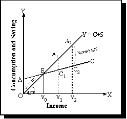
123

In the figure, when income increases from OY to OY1, Consumption also increases from EY0 to C1Y1, but the increase in consumption is less than the increase in income, i.e., C1Y1<CY. Similarly, when income increases from OY1 to OY2, consumption also increases from C1Y1 to C2Y2 and increased saving A2C2>A1C1.

Thus, Keynesian psychological law of consumption explains about the psychology of community towards expenditure pattern that the consumption function measures not only the amount spent on consumption but also the amount saved.

Consumption Function – Classical Theory of Employment – Concept of Consumption Function


CONCEPT OF CONSUMPTION FUNCTION

One of the important tools of the Keynesian Macroeconomics is the consumption function. Consumption function is simply a name for the general income-consumption relationship embodied in the Psychological law of Consumption given by Keynes. Keynesian general theory of employment is based on the consumption function. In economics, consumption means the amount spent on consumption at a given level of income. There is direct relationship between income and consumption. If income increases, the consumption also increases and vice-versa. The consumption function implies the whole of the schedule showing consumption expenditure at various level of income of the people. Thus, consumption function is also termed as ‘Propensity to Consume’. In short, the propensity to consume shows how the consumption expenditure varies with the change in income. According to K.K. Kurihara- “The propensity to consume is a schedule of expenditure at various income level”.

In the Keynesian theory, we are concerned not with the consumption of an individual consumer but with the sum of total consumption spending by all the individuals. The consumption function or propensity to consume refers to income-consumption relationship. It is a “functional relationship between two aggregates, i.e., total consumption and gross national income”. So, consumption is function of income. Because, the consumption changes with the change in income level. Thus, consumption depends upon the income level of the people. Symbolically, the consumption function is expressed as, C=f(Y), where, C is the consumption expenditure, Y is income and f is a function of (functional relationship)

So, the functional relationship between income and consumption is the consumption function. The consumption expenditure increases as increase in income. But consumption expenditure does not increase proportionately to the increase in the income. Consumption expenditure increases less than the proportionate increases in income. It is because people want to save part of income. Therefore, propensity to consume decreases as income increases because consumption will be less in proportion in relation to income.

The concept of consumption function can be explained by the help of psychological law of consumption developed by J.M. Keynor. According to this law people have a tendency to spend more on consumption when their income increases but not to same extent as income increase, because a part of income is saved. This can be illustrated as in the following table.

Schedule of Consumption

Rs. in Crores

Disposable Income (Y) Consumption Expenditure (C) Saving (S)

S = Y–C

0 20 –20
60 70 –10
120 120 0
180 170 10
240 220 20
300 270 30
360 320 40

In above consumption schedule, income increases at the some rate of Rs. 60 crores every time, but the consumption expenditure increases by only Rs. 50 crores every time. Therefore, when aggregate income increases, the aggregate consumption expenditure also increases. But, increase in consumption expenditure is less than proportionately increase in income, because some part of the increased income is saved.

Despite, the increase in income by Rs. 60 Crores every time and consumption expenditure increases by only Rs. 50 crores every time, but saving increases from 0 to Rs. 10, 20, 30 and 40 crores respectively. So, it can be clearly seen from the consumption schedule that as income increases, the consumption and saving both increases simultaneously.

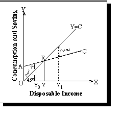
The concept of consumption function can also be illustrated graphically as follows:

zzzzz

In above given figure, consumption expenditure is presented along on OY–axis and level of income on OX–axis. The 45º line is joint curve showing the relation between income and consumption, which is started from origin. This 45° line shows the fact that income and consumption are equal to each other. That is, Y=C shows the fact that all the income of a consumer is used in consumption expenditure. AEC line represents tzhe consumption function. This line shows that as income increases the consumption expenditure also increases. But, this also shows that the consumption expenditure increases less proportionately as compared to increase in income. The line showing consumption function originates from the point A on OY–axis. This is because of consumption won’t be zero even if the income decreases to zero. Although, level of income is zero, the basic necessities must be fulfilled.

If income is less than the consumption, then this is fulfilled either by using the past savings or by taking loan. But, this gap between income and consumption decreases as the income increases. At OY level of income the consumption and income are equal to each other. In this situation, there will be neither any saving nor any defficiency. When income increases beyond this, the consumption will also increase, but not as fast as income increases because some part of the increased income will be saved. It can be expressed as:

Y = C+S

Where, Y = Income Level

C = Consumption Expenditure

S = Saving

Hence, consumption function measures not only the amount of income spent on consumption, but also the amount of income is saved.

Interdependence of micro and macro economics

Interdependence of micro and macro economics

Microeconomics and macroeconomics are two major branches of economics. So, they both are interdependent. Firm wise, individual wise, sector wise, district wise study of any economic activity is microeconomics. Overall study of all those study is macro study. So, any change in firm or individual or sector or district strongly affect to the national or macro economy. It way the policy made for national or macroeconomics brings the change in those different sectors or micro studies. So, close and particular analysis is microanalysis where as overall analysis of all economic activity is macro analysis. Economist Gardner Ackley has clearly said, “The relationship between macroeconomics and the theory of individual behavior is a two way street. On the one hand, microeconomic theory provides building blocks for the aggregate theories. But macroeconomics also contributes to microeconomic understanding.” Same way Edward Shapiro has made clearer with these words, “Strictly speaking, there is only one ‘economics’. Macroeconomic theory has a foundation in microeconomic theory and microeconomic theory has a foundation in macroeconomic theory.” The interdependence between these two branches of economics can be explained in following two topics:

  1. Dependence of microeconomics in macroeconomics

Microeconomics matters deeply depend upon the macroeconomic activity. For example, price, rate of interest, rate of profit, wages etc all are known as microeconomic topics. But all they depend upon macroeconomic behavior. Price, rate of interest, wage are determined by their demand and supply in country not by individual demand and supply. Same way, profit of any firm depends upon the nature of market, aggregate demand, national income, and general price level in economy. Aggregate demand, price level, national income, employment etc are deeply affected by macroeconomic fluctuations. Thus, change in macroeconomic indicators brings the change in microeconomic activities.

  1. Dependence of macroeconomics in microeconomics

Macroeconomics is overall study of microeconomic units. For example, employment of the country is the sum of all individual employment in different sectors. National income and national output is the sum of income and output of thousands of person and firms. Price level shows the average price, which comes through the appropriate calculation of prices of all transected commodities in the country in a fiscal year. Same way many theories of macroeconomics are derived from microeconomics theories. For example total consumption function and total investment function are based on the behavior of individual consumers and firms respectively. Thus, as a conclusion, it can be said that the study of macroeconomics comes throughout of microanalysis.

Being two broad branches of economics, each is paralyzed in the absence of other. P.A. Samuelson has clearly mentioned, “There is really no opposition between micro and macroeconomics. Both are absolutely vital. You are less than half educated, if you understand the one while being ignorant of the other.”

What is Business economics


What business economics is about? 

We discussed about various matters of economics under introduction topics. First unit- Introduction gives information about what is economics that means meaning of micro and macro-economics, their importance, types, limitations, their interdependence, their differences and many more. Now, it is time to know how business and economics are attached to each other. That is what we mean by business economics.

During production and distribution process, a business firm faces the various types of issues and problems. The first problem is which product is to be produced or which services are to be provided that is how to allocate the resources. The second problem is how the price and output level of commodity is determined that maximize profit or how to achieve the goals? It implies the efficient use of resources. Thus, a business firm has to be concerned about the application of economic theory during the decision making to solve such problems. The economics related to such business activities is known by business economics and, in advanced form, it is also known by managerial economics.

Business economics, on the one side, explains how the economic forces affect the working of the firm and on the other side, it also helps to predict the upcoming consequences of present business activities. Thus, it tells us the implemented policies by business managers to achieve business goals. To optimize the achievement, business managers apply optimization techniques like mathematical calculus, programming, statistical tools, geometrical diagrams etc. And other side, they apply various economic models. Thus, business economics can be described as the use of theories and techniques of modern economics for decisions making problems of business firms. Here, it should be noted that, business economics deals not only with profit earning private firms but it also deals with non-profit making organizations like colleges, universities, government etc.


What is Market ?


In common usage the word market designates a place where certain things are bought and sold. But when we talk about the word market in economics, we extend our concept of market well beyond the idea of a single place to which the householder goes to buy something. For our present purpose, we define a market as an area over which buyers and sellers negotiate the exchange of a well-defined commodity. For a single market to exist it must be possible for buyers and sellers to communicate with each other and to make meaningful deals other the whole market.

Definitions

Several economists have attempted to define the term market as used in economics. Some of them are as under: –

According to Prof. Chapman: “The term market refers not necessarily to a place but always to a commodity and the buyers and sellers who are in direct competition with one another.”

According to Curnot: “Economists understand by the term market not any particular market-place in which things are bought and sold, but the whole of any region in which buyers and sellers are in such free intercourse with one another that the price of the same goods tends to equality easily and quickly.”

In simple words, the term market refers to a structure in which the buyers and sellers of the commodity remain in close contact.


Features of the market 

On the basis above-mentioned definitions we can mention following main features of market:

  1. Buyers and Seller: Buyers and sellers are also essential for market. Without buyers and sellers the sale-purchase activity cannot be conducted which is essential part of a market.
  2. Commodity: For the existence of market, a commodity is essential which is to be bought and sold. There cannot be a market without commodity.
  • Area: There should be an area in which buyers and sellers of the commodity live in. It is not essential that the buyers and sellers should come to a particular place to transact the business.
  1. Close Contact: There should be close contact and communication between buyers and sellers. This communication may be established by any method. For example, in olden days this contact and communication was possible only when the buyers and sellers of a particular commodity could come at a particular place. But now with the developed means of communication physical presence of buyers and sellers at one particular place is not essential. They can contact with each other through letters, telegrams, telephones, etc. In the boundary of a market we include only those buyers and sellers who can maintain regular close contacts. For instance, India’s farmers have no close contacts with the consumers of England; hence though they are the buyers and sellers of grains yet do not come under the purview of a market.

There should be some competition among buyers and sellers of the commodity in a market.

Types of Market

A market can be divided on the basis of region (local, state and national market), period (very short period, short period and long period market) and competition. On the basis of competition there can be following types of market:

  1. Bilateral Monopoly. One buyer and one seller exist in the market.
  2. Pure Monopoly. One buyer and many sellers.
  • Pure Monopoly. One seller and many buyers.
  1. Two sellers and many buyers.
  2. A few sellers and many buyers.
  3. Monopolistic composition. Many buyers and many sellers’ produce producing differentiated products.
  • Perfect competition. Many buyers and sellers. Producers producing homogeneous or identical goods.
  • Imperfect competition. When competition is not complete and perfect due to one reason or the other, the market will be imperfect competitive market. All other types of market excluding perfect competition come under it. This market is wider than monopolistic competition.